Stitch single channel data
import paprica
import matplotlib.pyplot as plt
/opt/hostedtoolcache/Python/3.8.17/x64/lib/python3.8/site-packages/numpy/core/getlimits.py:500: UserWarning: The value of the smallest subnormal for <class 'numpy.float32'> type is zero.
  setattr(self, word, getattr(machar, word).flat[0])
/opt/hostedtoolcache/Python/3.8.17/x64/lib/python3.8/site-packages/numpy/core/getlimits.py:89: UserWarning: The value of the smallest subnormal for <class 'numpy.float32'> type is zero.
  return self._float_to_str(self.smallest_subnormal)
/opt/hostedtoolcache/Python/3.8.17/x64/lib/python3.8/site-packages/numpy/core/getlimits.py:500: UserWarning: The value of the smallest subnormal for <class 'numpy.float64'> type is zero.
  setattr(self, word, getattr(machar, word).flat[0])
/opt/hostedtoolcache/Python/3.8.17/x64/lib/python3.8/site-packages/numpy/core/getlimits.py:89: UserWarning: The value of the smallest subnormal for <class 'numpy.float64'> type is zero.
  return self._float_to_str(self.smallest_subnormal)
Let’s start by parsing a data-set:
path = '../../../tests/data/apr'
tiles = paprica.tileParser(path=path, ftype='apr', frame_size=512)
**********  PARSING DATA **********
../../../tests/data/apr
Tiles are of type apr.
13 tiles were detected.
4 rows and 4 columns.
***********************************
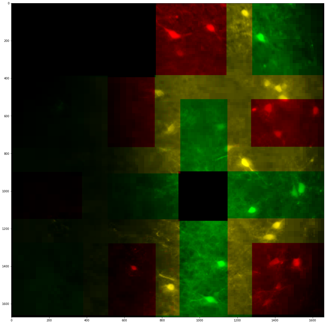
The data-set can then be quickly displayed by using the stitcher module using the expected tile position given the overlap and confirm that the data was parsed correctly.
stitcher_expected = paprica.tileStitcher(tiles, overlap_h=25, overlap_v=25)
stitcher_expected.compute_expected_registration()
To do so, we provide a lazy reconstructor with the stitcher to display a cross-section (or a max projection) of stitched data-set along any given dimension:
_ = stitcher_expected.reconstruct_slice(color=True, n_proj=10, progress_bar=False)

# The code below is only used to format the output image correctly for this tutorial and is not needed if used on your own machine
fig = plt.gcf()
fig.set_figheight(20)
fig.set_figwidth(20)
Error reading APR file: particle dataset 'particles' doesn't exist
---------------------------------------------------------------------------
ValueError                                Traceback (most recent call last)
Cell In[4], line 1
----> 1 _ = stitcher_expected.reconstruct_slice(color=True, n_proj=10, progress_bar=False)
      3 # The code below is only used to format the output image correctly for this tutorial and is not needed if used on your own machine
      4 fig = plt.gcf()

File /opt/hostedtoolcache/Python/3.8.17/x64/lib/python3.8/site-packages/paprica/stitcher.py:635, in baseStitcher.reconstruct_slice(self, loc, n_proj, dim, downsample, color, debug, plot, seg, progress_bar)
    604 """
    605 Reconstruct whole sample 2D section at the given location and in a given dimension. This function can also
    606 reconstruct a maximum intensity projection if `n_proj>0`.
   (...)
    631     Array containing the reconstructed data.
    632 """
    634 if dim == 0:
--> 635     return self._reconstruct_z_slice(z=loc, n_proj=n_proj, downsample=downsample, color=color,
    636                                      debug=debug, plot=plot, seg=seg, progress_bar=progress_bar)
    637 elif dim == 1:
    638     return self._reconstruct_y_slice(y=loc, n_proj=n_proj, downsample=downsample, color=color,
    639                                      debug=debug, plot=plot, progress_bar=progress_bar)

File /opt/hostedtoolcache/Python/3.8.17/x64/lib/python3.8/site-packages/paprica/stitcher.py:785, in baseStitcher._reconstruct_z_slice(self, z, n_proj, downsample, color, debug, plot, seg, progress_bar)
    782 level_delta = int(-np.sign(downsample) * np.log2(np.abs(downsample)))
    784 tile = self.tiles[0]
--> 785 tile.lazy_load_tile(level_delta=level_delta)
    786 if seg:
    787     tile.lazy_load_segmentation(level_delta=level_delta)

File /opt/hostedtoolcache/Python/3.8.17/x64/lib/python3.8/site-packages/paprica/loader.py:201, in tileLoader.lazy_load_tile(self, level_delta)
    198 if self.type != 'apr':
    199     raise TypeError('Error: lazy loading is only supported for APR data.')
--> 201 self.lazy_data = pyapr.reconstruction.LazySlicer(self.path, level_delta=level_delta, parts_name='particles',
    202                                                   tree_parts_name='particles')
    203 self.is_loaded = True

File /opt/hostedtoolcache/Python/3.8.17/x64/lib/python3.8/site-packages/pyapr/reconstruction/LazySlicer.py:72, in LazySlicer.__init__(self, file_path, level_delta, mode, parts_name, tree_parts_name, t, channel_name)
     70 tree_parts_name = tree_parts_name or get_particle_names(self.path, t=t, channel_name=channel_name, tree=True)[0]
     71 tree_parts_type = get_particle_type(self.path, t=t, channel_name=channel_name, parts_name=tree_parts_name, tree=True)
---> 72 self.tree_parts = type_to_lazy_particles(tree_parts_type)
     73 self.tree_parts.init_tree(self.aprfile, tree_parts_name, t, channel_name)
     74 self.tree_parts.open()

File /opt/hostedtoolcache/Python/3.8.17/x64/lib/python3.8/site-packages/pyapr/utils/types.py:63, in type_to_lazy_particles(typespec)
     61 if typespec in ('uint64', np.uint64):
     62     return LazyDataLong()
---> 63 raise ValueError(f'Type {typespec} is currently not supported. Valid types are \'uint8\', \'uint16\', '
     64                  f'\'uint64\' and \'float\' (\'float32\')')

ValueError: Type  is currently not supported. Valid types are 'uint8', 'uint16', 'uint64' and 'float' ('float32')
As you can see on the image above, there are doubling artifacts arising from tiles misalignment. To actively counteract these misalignments, the registration between tiles can be computed:
stitcher = paprica.tileStitcher(tiles, overlap_h=25, overlap_v=25)
stitcher.set_overlap_margin(10)
stitcher.compute_registration(progress_bar=False)

_ = stitcher.reconstruct_slice(color=True, n_proj=10, progress_bar=False)

# The code below is only used to format the output image correctly for this tutorial and is not needed if used on your own machine
fig = plt.gcf()
fig.set_figheight(20)
fig.set_figwidth(20)
Computing max. proj.: 100%|██████████| 13/13 [00:00<00:00, 27.44it/s]
Effective horizontal overlap: 25.29%
Effective vertical overlap: 24.71%

On the image above, the doubling artifacts are corrected. It is then possible to see the correct tile placement and save it. The ´database´ object is used by the rest of the pipeline by the viewer, merger and the segmenter to place tiles correctly.
print(stitcher.database)
# stitcher.save_database('path to saving location')
                               path  row  col    dH    dV   dD   ABS_H  \
0   ../../../tests/data/apr/0_2.apr    0    2   0.0   0.0  0.0   768.0
1   ../../../tests/data/apr/0_3.apr    0    3   3.0   0.0  0.0  1143.0
2   ../../../tests/data/apr/1_0.apr    1    0 -24.0  15.0  0.0     0.0
3   ../../../tests/data/apr/1_1.apr    1    1 -10.0  23.0  0.0   386.0
4   ../../../tests/data/apr/1_2.apr    1    2  -6.0  12.0  0.0   762.0
5   ../../../tests/data/apr/1_3.apr    1    3   8.0  12.0  0.0  1148.0
6   ../../../tests/data/apr/2_0.apr    2    0 -24.0  18.0  0.0     0.0
7   ../../../tests/data/apr/2_1.apr    2    1 -20.0  23.0  0.0   376.0
8   ../../../tests/data/apr/2_3.apr    2    3   9.0  21.0  0.0  1149.0
9   ../../../tests/data/apr/3_0.apr    3    0 -21.0  33.0  0.0     3.0
10  ../../../tests/data/apr/3_1.apr    3    1 -14.0  35.0  0.0   382.0
11  ../../../tests/data/apr/3_2.apr    3    2  -1.0  43.0  0.0   767.0
12  ../../../tests/data/apr/3_3.apr    3    3   9.0  30.0  0.0  1149.0

     ABS_V  ABS_D
0      0.0    0.0
1      0.0    0.0
2    387.0    0.0
3    395.0    0.0
4    384.0    0.0
5    384.0    0.0
6    762.0    0.0
7    767.0    0.0
8    765.0    0.0
9   1149.0    0.0
10  1151.0    0.0
11  1159.0    0.0
12  1146.0    0.0
Comparison of stitched and unstitched data
The cross sections can also be computed in other dimension (still using lazy loading) and compared between the stitched and unstitched data.
Before Stitching
_ = stitcher_expected.reconstruct_slice(dim=1, loc=650, color=True, n_proj=10, progress_bar=False)

# The code below is only used to format the output image correctly for this tutorial and is not needed if used on your own machine
fig = plt.gcf()
fig.set_figheight(20)
fig.set_figwidth(20)
Merging: 100%|██████████| 4/4 [00:00<00:00, 32.53it/s]

After Stitching
_ = stitcher.reconstruct_slice(dim=1, loc=650, color=True, n_proj=10, progress_bar=False)

# The code below is only used to format the output image correctly for this tutorial and is not needed if used on your own machine
fig = plt.gcf()
fig.set_figheight(20)
fig.set_figwidth(20)
Merging: 100%|██████████| 4/4 [00:00<00:00, 30.70it/s]

Before stitching
_ = stitcher_expected.reconstruct_slice(dim=2, loc=800, color=True, n_proj=10, progress_bar=False)

# The code below is only used to format the output image correctly for this tutorial and is not needed if used on your own machine
fig = plt.gcf()
fig.set_figheight(20)
fig.set_figwidth(20)
Merging: 100%|██████████| 6/6 [00:00<00:00, 53.54it/s]

After Stitching
_ = stitcher.reconstruct_slice(dim=2, loc=800, color=True, n_proj=10, progress_bar=False)

# The code below is only used to format the output image correctly for this tutorial and is not needed if used on your own machine
fig = plt.gcf()
fig.set_figheight(20)
fig.set_figwidth(20)
Merging: 100%|██████████| 6/6 [00:00<00:00, 47.24it/s]

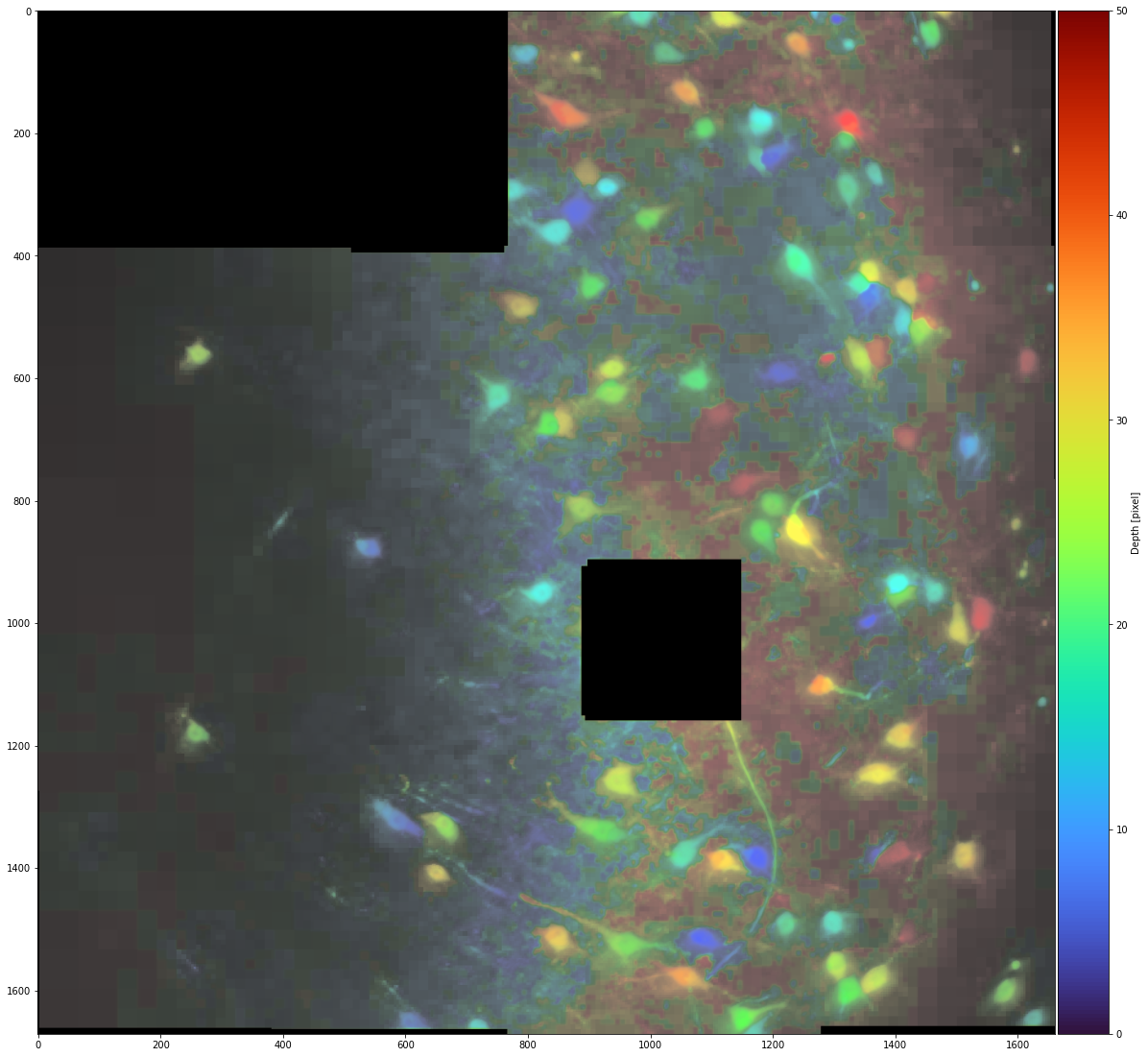
Color depth projection
It is also possible to display a color depth projection:
_ = stitcher.reconstruct_z_color(n_proj=50, progress_bar=False)

# The code below is only used to format the output image correctly for this tutorial and is not needed if used on your own machine
fig = plt.gcf()
fig.set_figheight(20)
fig.set_figwidth(20)
Merging: 100%|██████████| 13/13 [00:00<00:00, 23.34it/s]
